Analysis

Analysis based on Decision Trees, Random Forests, and Neural Networks.

Definitions

Let us first define some functions used throughout the notebook. We don’t include the imports for the sake of space, but please look at the notebook nbs/analysis.ipynb for details.

def draw_tree(t, df, size=10, ratio=0.6, precision=0, **kwargs):
    s=export_graphviz(t, out_file=None, feature_names=df.columns, filled=True, rounded=True,
                      special_characters=True, rotate=False, precision=precision, **kwargs)
    return graphviz.Source(re.sub('Tree {', f'Tree {{ size={size}; ratio={ratio}', s))

def cluster_columns(df, figsize=(10,6), font_size=12):
    corr = np.round(scipy.stats.spearmanr(df).correlation, 4)
    corr_condensed = hc.distance.squareform(1-corr)
    z = hc.linkage(corr_condensed, method='average')
    fig = plt.figure(figsize=figsize)
    hc.dendrogram(z, labels=df.columns, orientation='left', leaf_font_size=font_size)
    plt.show()

Let us also define some variables:

path = Path('data/datasets/autos.csv')
results_path = Path('results/used_cars')
results_path.mkdir (parents=True, exist_ok=True)

target_variable = 'sale_duration'
outliers = dict (numeric_variables_high=0.99,
                 numeric_variables_low=0.01,
                 date_created=True)
add_datepart_flag = True

cd ..

/home/jaumeamllo/workspace/mine/tabularml

Load data

The first step is to load the data and have a quick look at it:

df = pd.read_csv(path, encoding="ISO-8859-1", parse_dates=['dateCrawled', 'dateCreated', 'lastSeen'])

df.head()

	dateCrawled	name	seller	offerType	price	abtest	vehicleType	yearOfRegistration	gearbox	powerPS	model	kilometer	monthOfRegistration	fuelType	brand	notRepairedDamage	dateCreated	nrOfPictures	postalCode	lastSeen
0	2016-03-24 11:52:17	Golf_3_1.6	privat	Angebot	480	test	NaN	1993	manuell	0	golf	150000	0	benzin	volkswagen	NaN	2016-03-24	0	70435	2016-04-07 03:16:57
1	2016-03-24 10:58:45	A5_Sportback_2.7_Tdi	privat	Angebot	18300	test	coupe	2011	manuell	190	NaN	125000	5	diesel	audi	ja	2016-03-24	0	66954	2016-04-07 01:46:50
2	2016-03-14 12:52:21	Jeep_Grand_Cherokee_"Overland"	privat	Angebot	9800	test	suv	2004	automatik	163	grand	125000	8	diesel	jeep	NaN	2016-03-14	0	90480	2016-04-05 12:47:46
3	2016-03-17 16:54:04	GOLF_4_1_4__3TÜRER	privat	Angebot	1500	test	kleinwagen	2001	manuell	75	golf	150000	6	benzin	volkswagen	nein	2016-03-17	0	91074	2016-03-17 17:40:17
4	2016-03-31 17:25:20	Skoda_Fabia_1.4_TDI_PD_Classic	privat	Angebot	3600	test	kleinwagen	2008	manuell	69	fabia	90000	7	diesel	skoda	nein	2016-03-31	0	60437	2016-04-06 10:17:21

Cleaning and EDA

We first gather the numerical and categorical columns:

numerical_variables = [
    x for x in df.dtypes.index 
    if (str(df.dtypes[x]).startswith ('int') or str(df.dtypes[x]).startswith ('float')) and x != 'postalCode'
]
numerical_variables

['price',
 'yearOfRegistration',
 'powerPS',
 'kilometer',
 'monthOfRegistration',
 'nrOfPictures']

categorical_variables = set (df.columns).difference (numerical_variables)
categorical_variables

{'abtest',
 'brand',
 'dateCrawled',
 'dateCreated',
 'fuelType',
 'gearbox',
 'lastSeen',
 'model',
 'name',
 'notRepairedDamage',
 'offerType',
 'postalCode',
 'seller',
 'vehicleType'}

categorical_variables = categorical_variables.difference ({'dateCrawled', 'dateCreated', 'name', 'lastSeen'})
categorical_variables = list (categorical_variables)

Outliers

Next, we remove outliers found in the data. For that purpose, we first examine the statistics of numerical variables:

df.describe()

	price	yearOfRegistration	powerPS	kilometer	monthOfRegistration	nrOfPictures	postalCode
count	3.715280e+05	371528.000000	371528.000000	371528.000000	371528.000000	371528.0	371528.00000
mean	1.729514e+04	2004.577997	115.549477	125618.688228	5.734445	0.0	50820.66764
std	3.587954e+06	92.866598	192.139578	40112.337051	3.712412	0.0	25799.08247
min	0.000000e+00	1000.000000	0.000000	5000.000000	0.000000	0.0	1067.00000
25%	1.150000e+03	1999.000000	70.000000	125000.000000	3.000000	0.0	30459.00000
50%	2.950000e+03	2003.000000	105.000000	150000.000000	6.000000	0.0	49610.00000
75%	7.200000e+03	2008.000000	150.000000	150000.000000	9.000000	0.0	71546.00000
max	2.147484e+09	9999.000000	20000.000000	150000.000000	12.000000	0.0	99998.00000

• We see outliers in:

1. Price: minimum value 0, and maximum value > 2000M euros
2. Year of registration: minimum value 1000, and maximum value > 3000
3. Month of registration: minimum value 0
4. powerPS: minimum value 0, maximum value 20K

• We also see that nrOfPictures is always zero, so that it is not relevant

We have two possibilities:

1. Remove rows with outliers
2. Treat outlier values as missing values

In this analysis, we go for the second option.

Typical outlier detection methods:

1. Based on percentile
2. Based on z-score

In this analysis, we go for the first option:

df_clean = df.copy()
df_clean[numerical_variables] = df_clean[numerical_variables].apply (
    lambda x: x.mask ((x < x.quantile(outliers['numeric_variables_low'])) | (x > x.quantile(outliers['numeric_variables_high'])))
)

# see if there are rows that have all values missing and need to be removed, and
# check maximum ratio of missing values in one row
df_clean[numerical_variables].isna().all(axis=1).any(), df_clean[numerical_variables].isna().mean(axis=1).max()

(False, 0.5)

Remove nrOfPictures

We remove the column nrOfPictures, since it is not relevant:

df_clean = df_clean.drop (columns='nrOfPictures')
numerical_variables.remove ('nrOfPictures')

dateCreated

We examine the column dateCreated:

df_clean.dateCreated.max()-df_clean.dateCreated.min()

Timedelta('759 days 00:00:00')

The time span is more than 2 years. However, we see below that there are only few cases where the ad was posted more than few months ago, while the rest are just a few months old. To see that, we transform dateCreated to the offset in terms of number of months since the earliest ad in the dataset:

df_clean['offset_date'] = (df_clean['dateCreated']-df_clean['dateCreated'].min()).dt.days

df_clean.offset_date.hist()

<Axes: >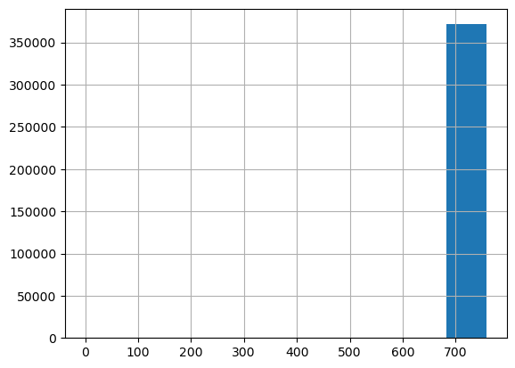

Clearly, almost all the ads are in one bin. Let’s look at this:

number_ads, bins = np.histogram (df_clean.offset_date)
pd.DataFrame ([number_ads, bins[1:]], index=['number_ads','bins'])

	0	1	2	3	4	5	6	7	8	9
number_ads	1.0	0.0	0.0	0.0	1.0	0.0	4.0	5.0	53.0	371464.0
bins	75.9	151.8	227.7	303.6	379.5	455.4	531.3	607.2	683.1	759.0

In the table above, we see that the last bin is where almost all the ads are, followed by the second to last bin, with few ads. From the 5th bin downwards, there are only 2 ads.

very_old_ads = df_clean[df_clean.offset_date < 450]
other_ads = df_clean[df_clean.offset_date >= 450]

print ('oldest ads created between: ', very_old_ads.dateCreated.min(),very_old_ads.dateCreated.max())

print ('remaining ads created between: ', other_ads.dateCreated.min(),other_ads.dateCreated.max())

oldest ads created between:  2014-03-10 00:00:00 2015-03-20 00:00:00
remaining ads created between:  2015-06-11 00:00:00 2016-04-07 00:00:00

We have four options:

- no outlier
- oldest (2014) is outlier
- two oldest (before mid year 2016) are outliers.
- all but the ones in the last two bins (with 53 and 371464 rows) are outliers 
- use a quantile as done for the other numerical variables.

In this analysis, we use the third option: treat the two oldest ads as two outliers:

if outliers['date_created']:
    df_clean = df_clean[df_clean.dateCreated >= '2015-06-01']

df_clean = df_clean.drop (columns = 'offset_date')

yearRegistration + monthRegistration

We use yearOfRegistration and monthOfRegistration to calculate the age of the vehicle, in number of months since the ad was posted. We first look if the outlier removal removed suspicious low and high values:

df_clean[['monthOfRegistration','yearOfRegistration']].describe().loc[['min','max']]

	monthOfRegistration	yearOfRegistration
min	0.0	1978.0
max	12.0	2018.0

There are still months with value 0, we treat them as missing values. We impute them using the middle of the year, month 6.

df_clean.loc [df_clean.monthOfRegistration==0, 'monthOfRegistration'] = 6

df_clean['age'] = pd.to_datetime(df_clean.dateCreated.max()) - pd.to_datetime ({
    'month': df_clean.monthOfRegistration,
    'year': df_clean.yearOfRegistration,
    'day': np.tile (15, df_clean.shape[0])}
)

df_clean['age'] = df_clean['age'].dt.days

numerical_variables.remove ('yearOfRegistration')
numerical_variables.remove ('monthOfRegistration')
numerical_variables.append ('age')

Target variable

df_clean[target_variable] = (df_clean ['lastSeen'] - df_clean['dateCreated']).dt.days

date information

Depending on whether the ad was posted on a weekend, on holidays, etc., more people might be able to look at it and it might be sold more quickly. We add this information here:

if add_datepart_flag:
    country_holidays = holidays.country_holidays('DE')
    df_clean['holidays'] = [int(day in country_holidays) for day in df_clean.dateCreated]
    df_clean['day_of_week'] = df_clean.dateCreated.dt.dayofweek.values

numerical_variables.append ('day_of_week')
categorical_variables.append ('holidays')

joblib.dump ([df_clean, numerical_variables, categorical_variables], results_path / 'df_clean.pkl')

['results/used_cars/df_clean.pkl']

Histograms

We look at the resulting histograms to see if there are clear outliers. This doesn’t seem to be the case.

df_clean['price'].hist()

<Axes: >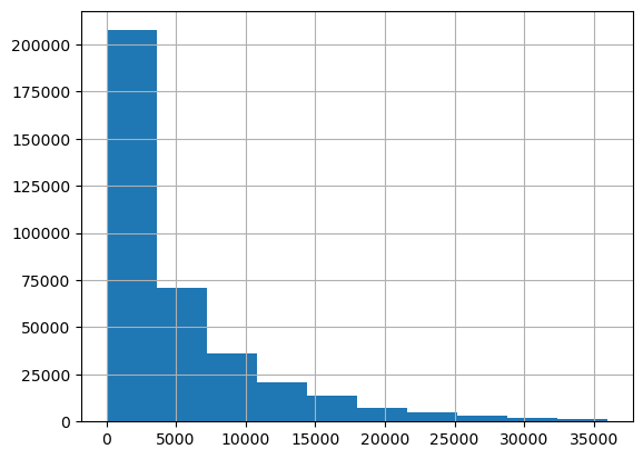

df_clean['age'].hist()

<Axes: >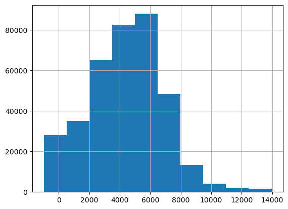

df_clean['powerPS'].hist()

<Axes: >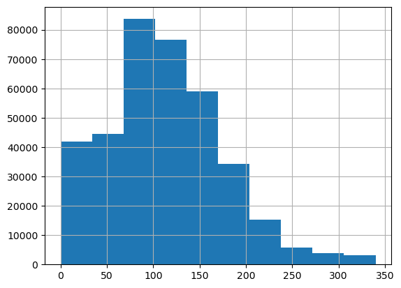

df_clean['kilometer'].hist()

<Axes: >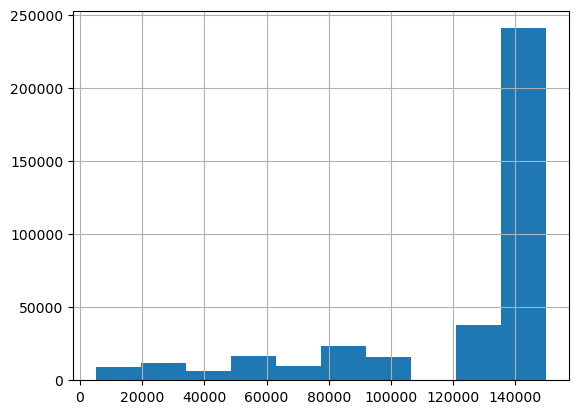

Split data and preprocess

The first step is to split the data in training and validation. For simplicity, e don’t use a test set here, although we should use it if we wanted to estimate the final accuracy after selecting our best model on the validation set.

from sklearn.model_selection import train_test_split

train_idx, valid_idx = train_test_split(np.arange(df_clean.shape[0]), test_size=0.30, random_state=42)
joblib.dump ([train_idx, valid_idx], results_path / 'indexes.pkl')

['results/used_cars/indexes.pkl']

The second step is to preprocess the data. We do that with the help of TabularPandas in the fastai library:

• Using Categorify, we replace columns in categorical_variables list with numeric categorical columns. We use just an discrete value instead of using a one-hot encoding. This tends to work better for decision trees and random forests, as explored in “Splitting on Categorical Predictors in Random Forests”

• Using FillMissing, we replace missing values with the median, and we create a boolean column that is True for any row where the value was missing

procs = [Categorify, FillMissing]
tabular = TabularPandas (df_clean, procs, categorical_variables, numerical_variables, y_names=target_variable, splits=(list(train_idx),list(valid_idx)))

path = Path('data/datasets')
joblib.dump (tabular, path / 'tabular.pkl')

['data/datasets/tabular.pkl']

Decision Tree

We start by fitting a very simple yet powerful type of model, the decision tree. A good characteristic of this type of model is that it is interpretable and allows to analyze the data and the important variables.

tabular = joblib.load (path / 'tabular.pkl')

X, y = tabular.train.xs, tabular.train.y
valid_X, valid_y = tabular.valid.xs, tabular.valid.y

Visualization

We can visualize on which basis the tree splits the data. We see that:

- The most important predictor is the `price`: the lower the price, the lower the duration of the sale. 
- The data where most errors happen is the one for large durations. This might be due to the few cases with a long duration, which could be considered almost outliers.

m = DecisionTreeRegressor(max_leaf_nodes=4)
m.fit (X, y);

draw_tree(m, X, size=10, leaves_parallel=True, precision=2)

Warning: Could not load "/home/jaumeamllo/miniconda3/envs/tsforecast/bin/../lib/graphviz/libgvplugin_pango.so.6" - It was found, so perhaps one of its dependents was not.  Try ldd.
Warning: no value for width of non-ASCII character 226. Falling back to width of space character

We can visualize the same using the dtreeviz library:

samp_idx = np.random.permutation(len(y))[:500]
viz = dtreeviz.model (m, X.iloc[samp_idx], y.iloc[samp_idx], feature_names=X.columns, target_name=target_variable)

viz.view (fontname='DejaVu Sans', scale=2, label_fontsize=16,
        orientation='LR')

/home/jaumeamllo/miniconda3/envs/tsforecast/lib/python3.10/site-packages/sklearn/base.py:420: UserWarning: X does not have valid feature names, but DecisionTreeRegressor was fitted with feature names
Warning: Could not load "/home/jaumeamllo/miniconda3/envs/tsforecast/bin/../lib/graphviz/libgvplugin_pango.so.6" - It was found, so perhaps one of its dependents was not.  Try ldd.
Warning: no value for width of non-ASCII character 226. Falling back to width of space character

Training

Let’s first start by training a full size decision tree.

dt_model = DecisionTreeRegressor()
dt_model.fit(X, y);

Evaluation

We use the root of the mean squared error as evaluation metric.

def r_mse (pred, y): 
    return round(math.sqrt(((pred-y)**2).mean()), 6)
def m_rmse (dt_model, X, y): 
    return r_mse(dt_model.predict(X), y)

Let’s see at the error on the training set:

m_rmse (dt_model, X, y)

0.283855

… and on the validation set:

m_rmse (dt_model, valid_X, valid_y)

11.614361

We can see that we are clearly overfitting. Let’s look at the number of leaves, and compare it against the total number of observations:

dt_model.get_n_leaves(), len(X)

(201472, 260068)

The number of leaves is similar to the number of observations. We need to reduce the size of the decision tree:

dt_model = DecisionTreeRegressor (min_samples_leaf=25)
dt_model.fit (tabular.train.xs, tabular.train.y)
m_rmse (dt_model, X, y), m_rmse(dt_model, valid_X, valid_y)

(7.683234, 8.817406)

We get a much better error on validation set, let’s see the number of leaves:

dt_model.get_n_leaves()

7949

Random Forest

We have built a baseline using Decision Trees. Let us explore now the use of Random Rorests

Training

def fitted_rf (X, y, n_estimators=128, max_features=0.5, min_samples_leaf=5, **kwargs):
    return RandomForestRegressor (
        n_jobs=-1, n_estimators=n_estimators, max_features=max_features,
        min_samples_leaf=min_samples_leaf, oob_score=True, **kwargs
    ).fit(X, y)

rf_model = fitted_rf (X, y);
joblib.dump (rf_model, results_path / 'rf_model1.pkl')

Evaluation

m_rmse (rf_model, X, y), m_rmse(rf_model, valid_X, valid_y), r_mse (rf_model.oob_prediction_, y)

(6.048382, 8.272029, 8.215691)

We see whether using another rule like the sqrt for calculating max_features per tree improves the model:

rf_model_2 = fitted_rf (X, y, max_features='sqrt');
m_rmse (rf_model_2, X, y), m_rmse(rf_model_2, valid_X, valid_y), r_mse(rf_model_2.oob_prediction_, y)

(6.649456, 8.296415, 8.233054)

It doesnt’ improve. We could play with the ratio of max features, min samples per leaf, and other hyper-parameters. We leave this as future work.

Visualization

Let’s see the impact of n_estimators on the performance:

import warnings
warnings.filterwarnings ('ignore')
preds = np.stack([t.predict(valid_X) for t in rf_model.estimators_])
plt.plot([r_mse(preds[:i+1].mean(0), valid_y) for i in range(128)]);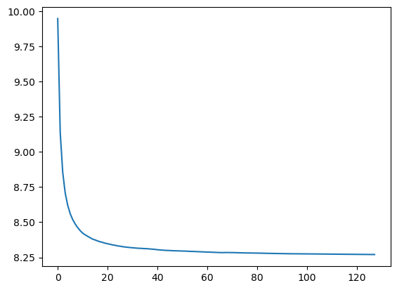

We see that the accuracy plateaus from 80 estimators onwards

Interpretation

Confidence

We look at the standard deviation of the predictions across the different trees. For those sales where there is low standard deviation, most of the trees agree on the sale duration estimate. This is useful in production, to maybe avoid providing a predition for those requests where there is little agreement on the sale duration.

preds = np.stack([t.predict(valid_X) for t in rf_model.estimators_])
preds_std = preds.std(0)

plt.hist (preds_std);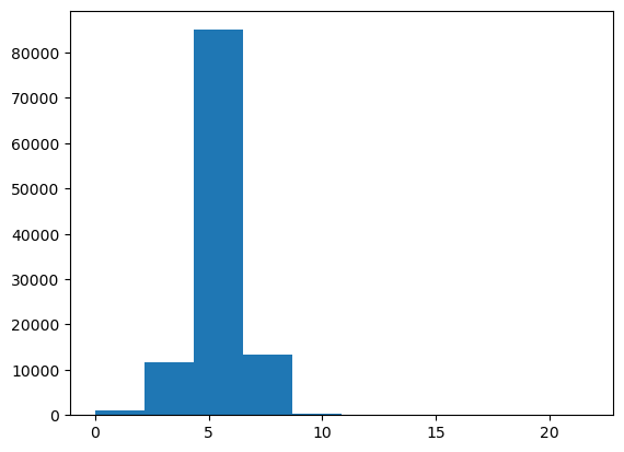

We see that there is in general high standard deviation for most sales, except for few cases.

Feature importance

Let’s look at what features are most important for the regression task:

def rf_feat_importance (rf_model, df):
    return pd.DataFrame({'cols':df.columns, 'imp':rf_model.feature_importances_}).sort_values('imp', ascending=False)

importance = rf_feat_importance (rf_model, X)
importance

	cols	imp
7	postalCode	0.193067
14	price	0.184392
17	age	0.153438
15	powerPS	0.099052
6	model	0.088209
0	brand	0.061477
18	day_of_week	0.060955
3	vehicleType	0.042012
16	kilometer	0.036495
9	abtest	0.023295
4	fuelType	0.016574
8	gearbox	0.015988
5	notRepairedDamage	0.015318
10	holidays	0.006917
11	price_na	0.001413
13	age_na	0.000947
12	powerPS_na	0.000451
1	seller	0.000000
2	offerType	0.000000

We see that the most important features are:

- postalCode: probably due to the higher density of population, and thus buyers, in certain areas.
- price: cheaper cars are sold faster.
- age: newer is better

Surprisingly, the day of the week plays a role even more important than the number of kilometers, to be sold faster, maybe because people look at ads more at certain days of the week.

Let’s look at the same graphically:

def plot_feature_importance (importance):
    return importance.plot('cols', 'imp', 'barh', figsize=(12,7), legend=False)

plot_feature_importance(importance);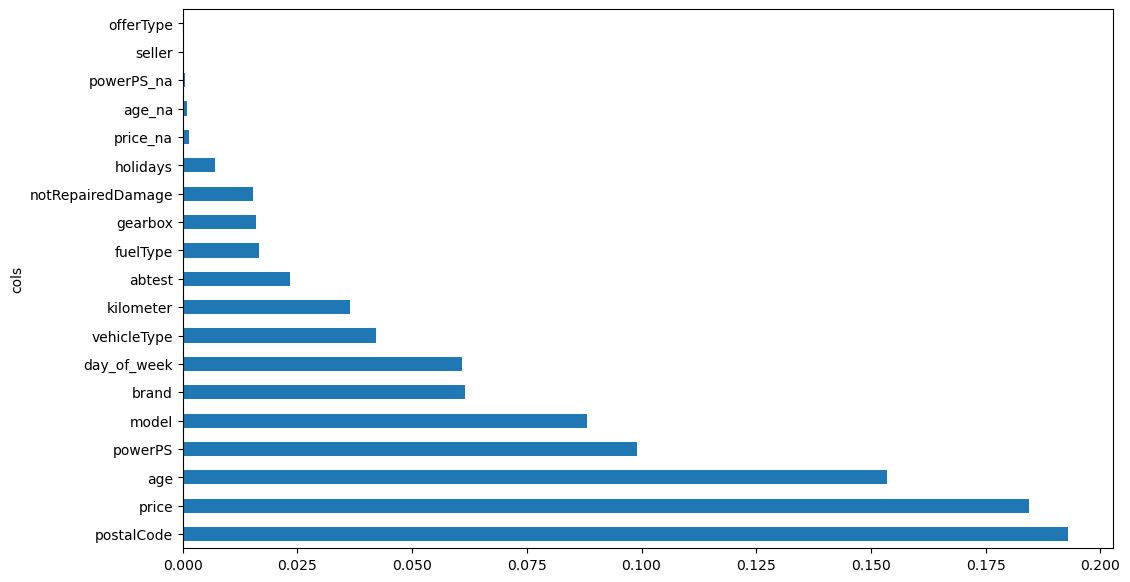

Removing variables

We see if we can improve the performance by removing those features that have very little importance and might be adding noise:

def evaluate_removing_variables (importance, X, y, valid_X, valid_y, threhsold):
    to_keep = importance[importance.imp>threhsold].cols
    X_imp = X[to_keep]
    valid_X_imp = valid_X[to_keep]

    rf_model = fitted_rf(X_imp, y)
    print (m_rmse(rf_model, X_imp, y), m_rmse(rf_model, valid_X_imp, valid_y), r_mse (rf_model.oob_prediction_, y))
    return rf_model, X_imp, valid_X_imp, to_keep

rf_model, X_imp, valid_X_imp, to_keep = evaluate_removing_variables (importance, X, y, valid_X, valid_y, 0.0001)
joblib.dump (rf_model, results_path / 'removing_low_importance.pkl')

6.045863 8.268369 8.211243

['results/used_cars/removing_low_importance.pkl']

There is almost no improvement, let’s see a bit more agressive pruning:

rf_model2, X_imp2, valid_X_imp2, to_keep2 = evaluate_removing_variables (importance, X, y, valid_X, valid_y, 0.001)

6.050095 8.272465 8.213242

rf_model2, X_imp2, valid_X_imp2, to_keep2 = evaluate_removing_variables (importance, X, y, valid_X, valid_y, 0.005)

6.010566 8.271691 8.210651

The best threshold seems to be 0.0001. Let’s use it and look at the feature importance again, after removing variables with low importance:

importance = rf_feat_importance(rf_model, X_imp)
plot_feature_importance(importance);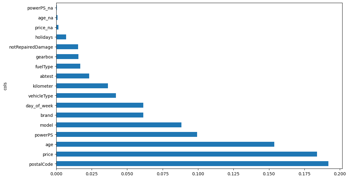

Removing redundant variables

We see if there are variables that might be closely correlated, in terms of ranking:

cluster_columns(X_imp)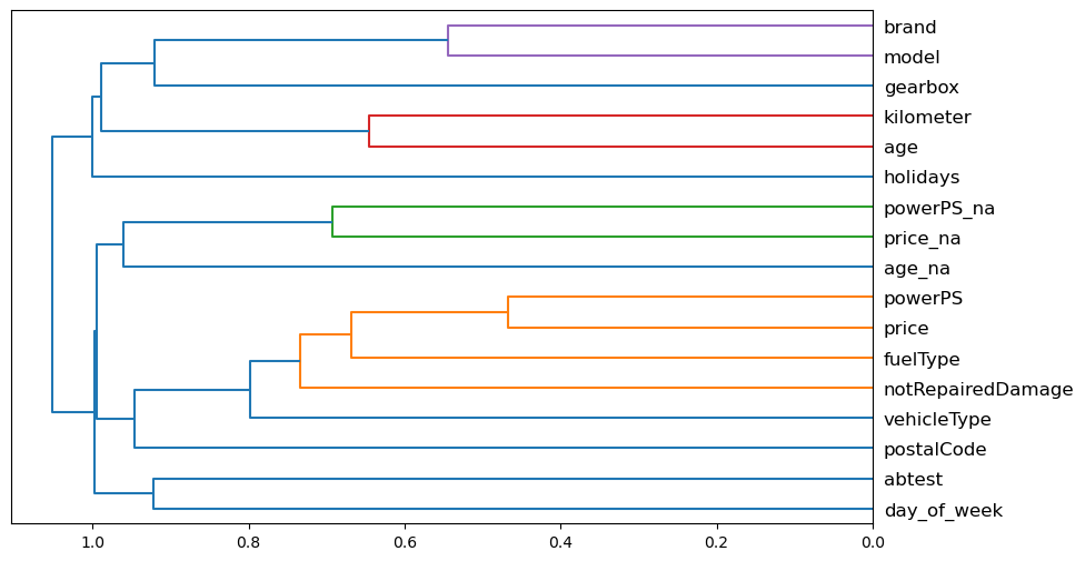

PowerPS and price seem to be quite correlated. We see what happens when we remove each of the variables in turn. To do it quickly, we use the out-of-bag score, by using a random forest where each tree is trained on a smaller subset of data, so that the out-of-bag score is measured on the remaining subset. This score indicates the generalization provided, being the higher the better.

def get_oob (df, y):
    m = RandomForestRegressor(n_estimators=40, min_samples_leaf=15,
        max_samples=50000, max_features=0.5, n_jobs=-1, oob_score=True)
    m.fit(df, y)
    return m.oob_score_

Let’s see the score of the original features:

def fitted_rf2 (X, y):
    return RandomForestRegressor (
        n_estimators=40, min_samples_leaf=15,
        max_samples=50000, max_features=0.5, n_jobs=-1, oob_score=True).fit(X, y)

original_oob = get_oob(X_imp, y)
original_oob

0.06008218588804892

oob_scores = {c:get_oob(X_imp.drop(c, axis=1), y) for c in (importance.cols)}
oob_scores

{'postalCode': 0.058280710022504234,
 'price': 0.0415493436634512,
 'age': 0.05244495695648832,
 'powerPS': 0.059019327633660135,
 'model': 0.0593482908544406,
 'brand': 0.058739696982127,
 'day_of_week': 0.05945691943436404,
 'vehicleType': 0.05943518125387026,
 'kilometer': 0.05984718680711576,
 'abtest': 0.06071818811404983,
 'fuelType': 0.060080938385732696,
 'gearbox': 0.06072952180624125,
 'notRepairedDamage': 0.06106010397906847,
 'holidays': 0.05685565776346668,
 'price_na': 0.060948957015006355,
 'age_na': 0.06027832457888893,
 'powerPS_na': 0.06106806907313633}

{k:oob_scores[k] for k in oob_scores if oob_scores[k] > original_oob}

{'abtest': 0.06071818811404983,
 'gearbox': 0.06072952180624125,
 'notRepairedDamage': 0.06106010397906847,
 'price_na': 0.060948957015006355,
 'age_na': 0.06027832457888893,
 'powerPS_na': 0.06106806907313633}

It seems that dropping the notRepairedDamage, abtest, and powerPS_na might be beneficial

def evaluate_removing_redundant (to_drop, X_imp, y, valid_X, valid_y):
    print ('OOB score: ', get_oob(X_imp.drop(to_drop, axis=1), y))
    X_final = X_imp.drop(to_drop, axis=1)
    valid_X_final = valid_X_imp.drop(to_drop, axis=1)
    rf_model = fitted_rf(X_final, y)
    print ('Regression errors: ', m_rmse(rf_model, X_final, y), m_rmse(rf_model, valid_X_final, valid_y), r_mse(rf_model.oob_prediction_, y))
    
    return rf_model, X_final, valid_X_final

rf_model, X_final, valid_X_final = evaluate_removing_redundant (['abtest', 'notRepairedDamage', 'powerPS_na'], X_imp, y, valid_X, valid_y)
joblib.dump ([rf_model, X_final, valid_X_final], results_path / 'removing_redundant.pkl')

OOB score:  0.0611047486037124
Regression errors:  6.050136 8.261787 8.202955

['results/used_cars/removing_redundant.pkl']

rf_model2, X_final2, valid_X_final2 = evaluate_removing_redundant (['notRepairedDamage', 'powerPS_na'], X_imp, y, valid_X, valid_y)

OOB score:  0.0606092565973716
Regression errors:  6.065446 8.26426 8.207189

rf_model2, X_final2, valid_X_final2 = evaluate_removing_redundant (['notRepairedDamage'], X_imp, y, valid_X, valid_y)

OOB score:  0.060027249156653584
Regression errors:  6.03148 8.262977 8.207328

rf_model2, X_final2, valid_X_final2 = evaluate_removing_redundant (['abtest'], X_imp, y, valid_X, valid_y)

OOB score:  0.060528790706093516
Regression errors:  6.037068 8.266976 8.205677

We select the model without [‘abtest’, ‘notRepairedDamage’, ‘powerPS_na’]. The result is slightly better, with lower number of variables, which tends to be good.

Neural Network

We use a similar preprocessing as the one used for RF, but with two important differences: - The numerical variables are standard normalized. - The categorical variables will be passed to an embedding layer in the Neural Network, which maps discrete integers to embeddings that have been learned to optimally represent each category in the variable. This tends to be a bit more effective and efficient than using one-hot-encoding.

selected_columns = set (X_final.columns).intersection(df_clean.columns)
df_nn = (df_clean[list(selected_columns) + [target_variable]]).copy()
df_nn[target_variable] = df_nn[target_variable].astype (np.float32)
categorical_variables = set (selected_columns).intersection (categorical_variables)
numerical_variables = set (selected_columns).intersection (numerical_variables)
procs = [Categorify, FillMissing, Normalize]
tabular = TabularPandas (df_nn, procs, list(categorical_variables), list(numerical_variables), y_names=target_variable, splits=(list(train_idx),list(valid_idx)))

We use a relatively high batch-size due to the fact that tabular data does not occupy much memory.

dls = tabular.dataloaders(1024)
y = tabular.train.y
learn = tabular_learner(dls, y_range=(np.floor(y.min()), np.ceil(y.max())), layers=[500,250],
                        n_out=1, loss_func=F.mse_loss)
learn.lr_find()

SuggestedLRs(valley=0.001737800776027143)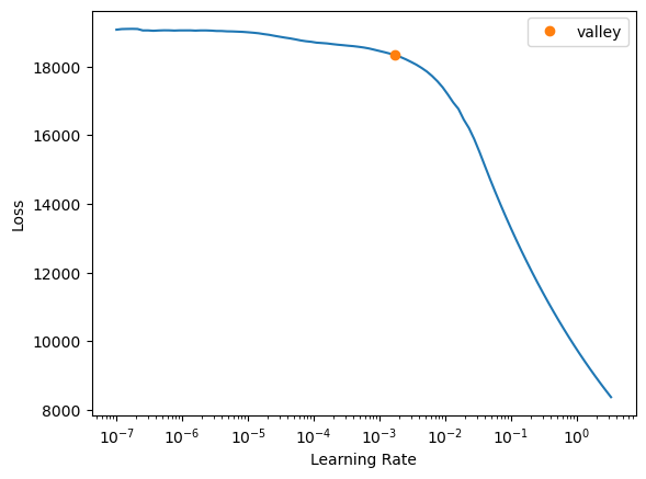

We try first with learning rate 1e-2 and 10 epochs:

learn.fit_one_cycle(10, 1e-2)

epoch	train_loss	valid_loss	time
0	602.610474	76.169884	00:11
1	78.452293	79.093147	00:10
2	72.395233	75.213257	00:10
3	68.382301	73.556313	00:10
4	64.683945	75.480438	00:10
5	61.083923	77.244652	00:10
6	50.728420	79.223137	00:11
7	43.104126	84.684929	00:10
8	34.933899	85.208206	00:10
9	30.915373	87.217155	00:10

We see that something close to 4 or 5 epochs is better

learn = tabular_learner(dls, y_range=(np.floor(y.min()), np.ceil(y.max())), layers=[500,250],
                        n_out=1, loss_func=F.mse_loss)
learn.fit_one_cycle(4, 1e-2)
preds, targs = learn.get_preds()
r_mse (preds,targs)

epoch	train_loss	valid_loss	time
0	345.358978	78.925217	00:11
1	74.916069	75.385986	00:10
2	65.404991	74.644577	00:10
3	51.674995	76.773880	00:11

8.762071

The validation error is 8.76, bigger than the one obtained by the RF. Let’s see with a lower learning rate:

learn2 = tabular_learner(dls, y_range=(np.floor(y.min()), np.ceil(y.max())), layers=[500,250],
                        n_out=1, loss_func=F.mse_loss)
learn2.fit_one_cycle(10, 1e-3)

epoch	train_loss	valid_loss	time
0	12781.711914	7655.472656	00:11
1	333.679382	107.907936	00:11
2	68.636696	75.976501	00:11
3	60.806812	77.812447	00:10
4	54.039669	81.903381	00:10
5	46.701462	79.440315	00:10
6	37.569061	79.386604	00:10
7	29.916273	80.873795	00:10
8	24.533495	81.103035	00:11
9	21.414110	81.744980	00:10

We see that the loss is not better than using a bigger learning rate. Let’s see even bigger:

learn2 = tabular_learner(dls, y_range=(np.floor(y.min()), np.ceil(y.max())), layers=[500,250],
                        n_out=1, loss_func=F.mse_loss)
learn2.fit_one_cycle(4, 1e-1)

epoch	train_loss	valid_loss	time
0	198.138016	131.202820	00:10
1	75.276131	75.907112	00:11
2	113.341293	151.957809	00:11
3	150.795166	151.957809	00:10

Clearly, the best learning rate seems to be 0.01

We could now examine other hyper-parameters, like regularization, dropout, adding more layers or units per layer, adding batch-normalization, etc.

Ensemble of RF and NN

We see if using an ensemble of RF and NN improves the results:

preds, targs = learn.get_preds()

rf_preds = rf_model.predict(valid_X_final)
ens_preds = (to_np(preds.squeeze()) + rf_preds) /2
r_mse(ens_preds,valid_y)

8.339824

While it improves the result of using NN, using RF alone seems to be a better option in this data.

Future lines of work

• As indicated above, we should now examine other hyper-parameters, like regularization, dropout, adding more layers or units per layer, adding batch-normalization, etc.
• Given that a random forest seems to be the best type of model for this data, it is a good idea to explore using XGBoost, CatBoost, or other types of tree ensembles.